0.原起 🔗
本新手打算整理一下建模型的基本方法,做点系统性的梳理认识下自身的不足,查漏补缺。不过并不打算一篇笔记写完全部,先初步写个非常基础的做二分类的建模流程,随后慢慢对模型可解释性、特征工程、效果验证等几方面内容单独写写。另外,虽然对 caret、mlr3 早有耳闻,但本新手都没接触过,有很多很优秀的方法和包都听说过但一直没来得及学习,希望未来的日子可以好好学学。
这篇笔记使用的 R 包如下:
- data.table:数据处理。
- DataExplorer:数据探索,主要用来批量绘图,由于此包依赖 ggplot2,数据量大了出图慢。
- echarts4r/DT:由于平时工作用的是 Rstudio Server,服务器上没有装 DataExplorer 这个包,实际上更多用基础的图表包来探索数据。
- scorecard:计算IV值,WOE转换,绘制 ROC曲线、K-S 曲线图。
- xgboost:训练模型。
1.数据集介绍 🔗
这是一个典型的用于做二分类预测的数据集,是在 Kaggle 上随意找的1,地址是https://www.kaggle.com/datasets/ifteshanajnin/carinsuranceclaimprediction-classification。
建模场景是:根据车险保单的车辆信息预测未来6月内是否会出险理赔。训练集有58592条数据,测试集有39063条数据,其中训练集有结果标签,而测试集无。
-
数据介绍
- 没有任何时间相关字段
- 没有缺失值,也没有系统误差造成的异常值
- 仅有车辆本身相关信息,没有任何与投保人自身属性或行为相关信息
- 也没有保单相关信息,如保费、保额、险类等。车险保费定价和有无出险理赔过相关,保费保额也是能反映出一些车辆的信息的。
-
字段介绍
- is_claim:结果标签,投保人未来6月内是否提出索赔
- policy_id:保单投保人唯一标识
- policy_tenure:保单期限
- age_of_car:车龄(按年,标准化处理后)
- age_of_policyholder:投保人年龄(按年,标准化处理后)
- area_cluster:投保人所在区域(重新编码处理后)
- population_density:城市人口密度(投保人城市)
其他字段
- make:汽车制造商的编码
- segment:汽车车型(A/ B1/ B2/ C1/ C2)(C1指手动挡小型汽车,C2指自动挡小型汽车,B1指中型客车,B2指大型货车,A1指大型客车)
- model:汽车的某种类型编码(从M1到M9分别限定了车辆载客座位数、载货总质量)
- fuel_type:汽车使用的燃料类型
- max_torque:汽车产生的最大扭矩
- max_power:汽车产生的最大功率
- engine_type:汽车发动机类型
- airbags:车内安全气囊数量
- is_esc:是否存在电子稳定控制系统(ESC)
- is_adjustable_steering:汽车方向盘是否可调整
- is_tpms:是否存在轮胎压力监测系统(TPMS)
- is_parking_sensors:是否存在停车传感器
- is_parking_camera:是否存在停车摄像头
- rear_brakes_type:汽车制动器类型
- displacement:汽车发送机排量
- cylinder:汽车发送机气缸数
- transmission_type:汽车变速器类型
- gear_box:车内齿轮数
- steering_type:汽车动力转向类型
- turning_radius:车辆转弯所需米数
- length:汽车长度
- width:汽车宽度
- height:汽车高度
- gross_weight:汽车最大载重
- is_front_fog_lights:是否有前雾灯
- is_rear_window_wiper:是否有后窗雨刷器
- is_rear_window_washer:是否有后窗清洗器
- is_rear_window_defogger:是否有后窗除雾器
- is_brake_assist:是否有制动辅助功能
- is_power_door_locks:是否有电动门锁
- is_central_locking:是否能中央控锁
- is_power_steering:是否能动力转向
- is_driver_seat_height_adjustable:是否可调整驾驶座高度
- is_day_night_rear_view_mirror:是否有后视镜
- is_ecw:是否有发动机检查警告(ECW)
- is_speed_alert:是否有速度报警
- ncap_rating:安全评级
保单期限(policy_tenure)这个字段有点奇怪,一般车险的保险保障期限都是一年,而数据集中做过标准化处理的保单期限分布在0.002735至1.396641之间。猜测这个字段的含义可能是一张保单未来剩余的保障期限,不然的话也可能是数据中混合了多种不同的车险险类。
2.探索性数据分析 🔗
在正式开始探索数据之前,需要先了解一下数据的基本概况。比如数据中好坏样本的比例,比例越失衡,建模型难度越高。要是碰到坏样本占比在千分之一或万分之一的情况,可能得先考虑清楚这份数据到底适不适合建立一个二分类的模型,如果不做二分类的话,是不是做异常检测更合适。另外,在建模型之前,确定一个清晰明确的验证目标,以及在上线后始终保持逻辑一致的标签定义,是更重要的事。比如先厘清这份数据的预测目标的标签定义为何是“未来6月内是否提出理赔”,如果只是预测短期出险的话为何是“6月内”而不是“3月内”或“1年内”,这里“理赔”的含义是否包含保险金欺诈。
-
查看训练集标签
0:1 = 54844:3748,整体理赔比例是6.39%,属于非平衡数据集。 -
一般需要看看按年、按月等不同时间维度的数据量变化趋势,比对一下各年数据差异。由于此数据集中没有时间字段,所以暂略。
-
看看有无拆分子模型的必要。一般越平衡的数据,建模越容易。如果数据拆分后,好坏样本比例差异很大,不妨一试。
-
看看数据缺失情况,若有,可删、可填补。有没有异常值,若有,可删、可修正。
library(data.table)
library(echarts4r)
library(DT)
library(scorecard)
library(xgboost)
library(DataExplorer)

train <- fread('baseline1/train.csv')
test <- fread('baseline1/test.csv')

train$is_claim <- as.numeric(train$is_claim)

train$type <- "train"
test$type <- "test"
test$is_claim <- NA

data <- rbind(train, test)

#最大扭矩、最大功率分别拆成两个字段
data$max_power_1 <-
  sapply(strsplit(as.character(data$max_power), 'bhp@'), "[", 1)
data$max_power_2 <-
  gsub("rpm", "", gsub("^.+bhp@", "", data$max_power))

data$max_torque_1 <-
  sapply(strsplit(data$max_torque, 'Nm@'), "[", 1)
data$max_torque_2 <-
  gsub("rpm", "", gsub("^.+Nm@", "", data$max_torque))

# 根据字段含义,部分字段可统一转换为因子型
char <- c(
  'area_cluster','make','segment','model','fuel_type','max_torque','max_power','engine_type','is_esc','is_adjustable_steering',
  'is_tpms','is_parking_sensors','is_parking_camera','rear_brakes_type','transmission_type','gear_box','steering_type','is_front_fog_lights',
  'is_rear_window_wiper','is_rear_window_washer','is_rear_window_defogger','is_brake_assist','is_power_door_locks','is_central_locking',
  'is_power_steering','is_driver_seat_height_adjustable','is_day_night_rear_view_mirror','is_ecw','is_speed_alert','ncap_rating','type')

# 根据字段含义,部分字段可统一转换为数值型
num <- c(
  'policy_tenure','age_of_car','age_of_policyholder','population_density','airbags','displacement','cylinder','turning_radius',
  'length','width','height','gross_weight','max_power_1','max_power_2','max_torque_1','max_torque_2')

# head(data[,..num])
# head(data[,..char])
data <-
  data[, (char) := lapply(.SD, as.factor), .SDcols = char][, (num) := lapply(.SD, as.numeric), .SDcols = num]

# sapply(data, function(x) sum(is.na(x))) # 计算缺失值
# summary(data)
2.1.批量查看数据分布 🔗
用 DataExplorer 包来批量查看数据的一些基本情况。一番比较查看后,很容易发现,这份数据的训练集和测试集的数据分布相当一致,绝大多数字段的理赔比例都分布得很均匀,构造特征的空间不大。
- 数值型数据查看直方图或箱线图
- 类别型数据查看柱状图、条形图、饼图
- 比对一下训练集、测试集数据差异
plot_bar(data[, ..char])
plot_histogram(data[, ..num])

# 比较训练集、测试集数据分布有没有差异
# plot_bar(data[type == 'train', ..char])
# plot_bar(data[type == 'test', ..char])
# plot_histogram(data[type == 'train', ..num])
# plot_histogram(data[type == 'test', ..num])

# 比较训练集、测试集在数据取值比例上有无差异
plot_bar(data[, ..char], by = "type")
plot_boxplot(data, by = "type")

# 查看训练集中各字段在标签上的比例有无差异
train$is_claim <- as.factor(train$is_claim)
plot_bar(train, by = "is_claim")
plot_bar(train, by = "is_claim", by_position = "dodge")
去年看到一种叫做对抗验证的思路,用于确认训练集测试集的数据分布是否一致,大意是将数据来源于训练集还是测试集作为标签来训练模型,如果模型的 AUC 值接近0.5,那么训练集测试集的数据分布便算是一致的。
2.2.进一步探索 🔗
如果是分析熟悉的业务数据,可以直接根据数据表现来验证猜想。但是笔者对车辆性能一点都不熟,两眼一摸瞎,干脆先算一下所有特征的 IV 值(Information Value,信息值),看看有没有哪些特征对结果影响大点。
iv <- scorecard::iv(data[type=='train', -c('policy_id', 'type')], y = 'is_claim')
datatable(iv)
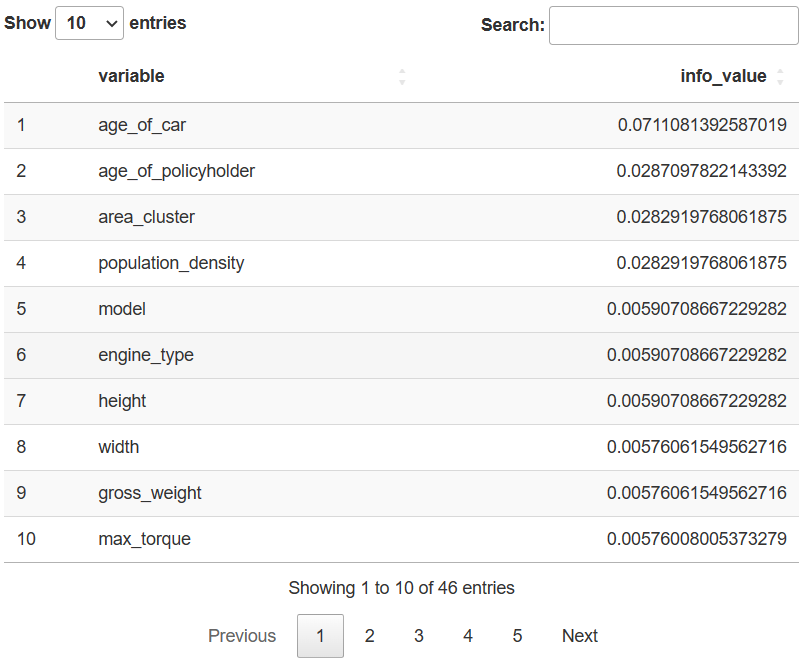
只有四个 IV 值超过0.02的字段,其中投保人所在区域(area_cluster)和城市人口密度(population_density)的 IV 值居然完全相等,两个字段的取值可能是一一对应的。还有不少 IV 值小于0.02的字段,其 IV 值也完全一致,那些字段的具体取值大概都是一一对应的。
table(data$population_density, data$area_cluster)
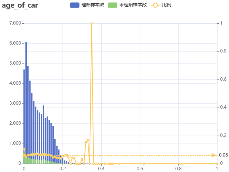
- age_of_car:数值型,车龄(按年,标准化处理后)。怎么车龄为0的客户理赔比例最高呢?
折叠代码块
tmp <- data[type == 'train', by = .(age_of_car), .(
    cnt = uniqueN(policy_id),
    cnt_0 = uniqueN(policy_id[is_claim == '0']),
    cnt_1 = uniqueN(policy_id[is_claim == '1'])
  )][, ':='(bili = round(cnt_1 / cnt, 4))]

tmp |>
  e_charts(age_of_car) |>
  e_bar(cnt_0,
        name = '理赔样本数',
        stack = 'group',
        y_index = 0) |>
  e_bar(cnt_1,
        name = '未理赔样本数',
        stack = 'group',
        y_index = 0) |>
  e_line(bili, name = '比例', y_index = 1) |>
  e_tooltip(trigger = 'axis') |>
  e_title(text = 'age_of_car') |>
  e_x_axis(max = 1) |>
  e_mark_line("比例", data = list(yAxis = 0.0639))
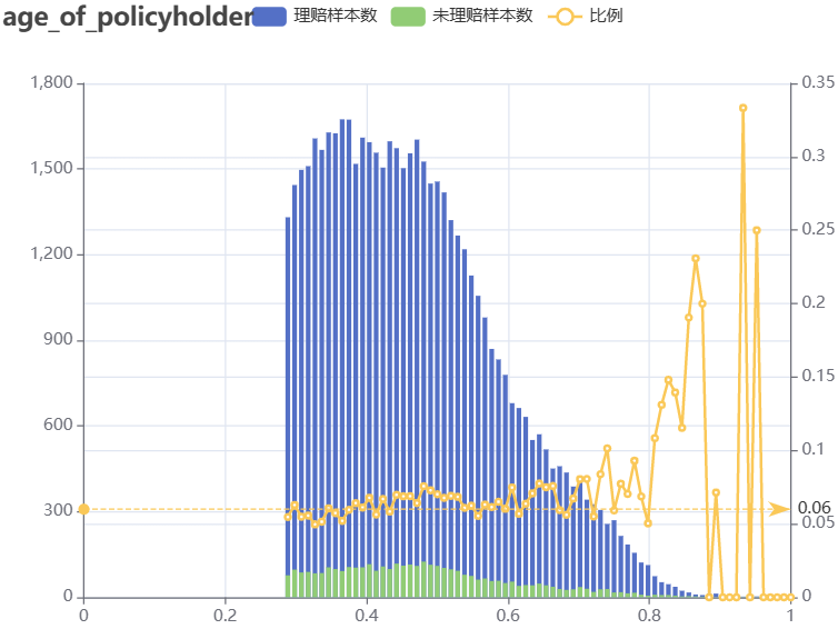
- age_of_policyholder:数值型,投保人年龄(按年,标准化处理后)。随着投保人年龄增长,理赔比例在波动……
折叠代码块
tmp <- data[type == 'train', by = .(age_of_policyholder), .(
    cnt = uniqueN(policy_id),
    cnt_0 = uniqueN(policy_id[is_claim == '0']),
    cnt_1 = uniqueN(policy_id[is_claim == '1'])
  )][, ':='(bili = round(cnt_1 / cnt, 4))]

tmp |>
  e_charts(age_of_policyholder) |>
  e_bar(cnt_0,
        name = '理赔样本数',
        stack = 'group',
        y_index = 0) |>
  e_bar(cnt_1,
        name = '未理赔样本数',
        stack = 'group',
        y_index = 0) |>
  e_line(bili, name = '比例', y_index = 1) |>
  e_tooltip(trigger = 'axis') |>
  e_title(text = 'age_of_policyholder') |>
  e_x_axis(max = 1) |>
  e_mark_line("比例", data = list(yAxis = 0.0639))
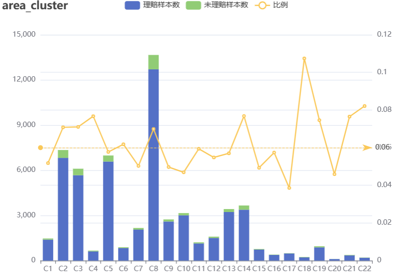
- area_cluster:字符型,投保人所在区域(重新编码处理后)。部分区域样本数远超其他。
折叠代码块
tmp <-
  data[type == 'train', by = .(area_cluster), .(
    cnt = uniqueN(policy_id),
    cnt_0 = uniqueN(policy_id[is_claim == '0']),
    cnt_1 = uniqueN(policy_id[is_claim == '1'])
  )][, ':='(bili = round(cnt_1 / cnt, 4))]

tmp |>
  e_charts(area_cluster) |>
  e_bar(cnt_0,
        name = '理赔样本数',
        stack = 'group',
        y_index = 0) |>
  e_bar(cnt_1,
        name = '未理赔样本数',
        stack = 'group',
        y_index = 0) |>
  e_line(bili, name = '比例', y_index = 1) |>
  e_tooltip(trigger = 'axis')|>
  e_title(text = 'area_cluster')|>
  e_mark_line("比例", data = list(yAxis = 0.0639)) |>
  e_x_axis(axisLabel = list(interval = 0))
- 维度交叉看看,比如投保人所在区域和投保人年龄或车龄的分布,暂不展开。这里就是看看整体数据中有没有哪一部分的理赔比例高出6.39%。如果能找出这样的一个组成部分,且其背后代表的规律能始终保持一致,那么大概率就是找出来一个很有用的特征。笔者的个人习惯是很喜欢分析数据的组成成分和变化趋势……
3.特征筛选 🔗
在筛选特征之前,先得在原数据基础上做充分的探索,在分析的基础上构造新特征。一般情况下,需要上线应用的模型,在构造新特征有几点需要特别注意:
-
不能泄露标签。当前取用历史数据建模预测未来时,所使用的数据应能还原历史。
-
谨慎地验证特征的稳定性。在探索数据时,应谨慎观察分析得到的数据规律是否能在多数情况下保持一致。建模型实际上就是探寻数据中隐藏的规律,积累大量的偶然性规律后虽不能直接得到必然性结论,但可以发现或者说预测出提高偶然规律的概率。不稳定的特征如果只是偶然看起来管用,实则就是无用。
-
构造的特征太多,后面筛选特征时也麻烦。
-
在训练数据和验证数据中要保持各方面一致。举个奇葩例子,如果某些特征刚好只在保留的时间外验证数据中效果极好,可能让验证效果看起来很好。
3.0.构造特征 🔗
由于这份数据构造特征的空间很有限,加上笔者水平也很有限,本小节写得十分简略。
-
方法一:针对类别型特征,将标签替换为数字后两两相乘,或者直接把各字段中的字符串拼接在一起,看能否得到 IV 值超过0.02的新特征。
-
方法二:针对数值型特征,计算不同维度下或者不同维度交叉组合下的件数(count)、金额(sum),或计算最大值、最小值、平均值、中位数等。
-
方法三:结合对数据的探索和认知来构造新特征。比如仔细看看特征两两组合以后,哪些组合情况下理赔比例高于总体样本,且占比也不低(约大于0.1)的,然后单独构造新特征。依此方法共构建了 f1/f2/f3/f4/f5等5个新特征。
折叠代码块
# 方法三 举个栗子
# tmp <-
#   data[type == 'train', by = .(area_cluster, make), .(
#     cnt = uniqueN(policy_id),
#     cnt_0 = uniqueN(policy_id[is_claim == '0']),
#     cnt_1 = uniqueN(policy_id[is_claim == '1'])
#   )][, ':='(bili1 = round(cnt_1 / cnt, 4),
#             bili2 = round(cnt / 58592, 4))]
#
# datatable(tmp,
#           filter = list(
#             position = 'top',
#             # 可选参数值有"none", "bottom", "top"
#             clear = TRUE,
#             # 是否展示在筛选框中输入过滤条件后的清除按钮
#             plain = FALSE
#           )) |>
#   formatStyle(columns = c(6), color = styleInterval(c(0.0639), c('black', 'red'))) |>
#   formatStyle(columns = c(7), color = styleInterval(c(0.1), c('black', 'green')))

data$f1 <- ifelse(data$age_of_car == 0, 1, 0)

data$f2 <-
  ifelse(data$area_cluster %in% c('C2', 'C3', 'C4', 'C8', 'C14', 'C18', 'C19', 'C21', 'C22'), 1, 0)

data$f3 <-
  ifelse((
    data$area_cluster %in% c('C8', 'C2', 'C14') &
      data$segment %in% c('B2', 'C2')) |
    (data$area_cluster == 'C3' &
       data$segment %in% c('A', 'B2')) |
    (data$area_cluster == 'C8' &
       data$segment == 'C1') |
    (data$area_cluster == 'C12' & data$segment == 'B2'), 1, 0)

data$f4 <-
  ifelse((
    data$make == '1' &
      data$area_cluster %in% c('C8', 'C3', 'C2', 'C14', 'C19', 'C4')) |
    (data$make == '3' & data$area_cluster %in% c('C8', 'C2', 'C14')), 1, 0)

data$f5 <-
  ifelse((
    data$area_cluster %in% c('C8', 'C2', 'C3', 'C14') &
      data$fuel_type %in% c('Petrol', 'Diesel')) | (data$area_cluster %in% c('C3', 'C14') &
         data$fuel_type == 'CNG'), 1, 0)
3.1.数据分箱 🔗
使用 scorecard 包做数据分箱,就是将特征进行离散化处理,比如将连续型特征处理成离散型;或者将类别较多的特征使其部分类别合并,从而处理成类别更少的。这样做的好处有几点:一是特征更稳定,模型也更稳定;二是离散化的特征更好解释;三是可以提升计算速度,比如说如果手动用笔计算两个矩阵相乘,肯定是更稀疏或者更简单的矩阵算起来更快的。
####
#1.进行WOE转换时,需要先去掉一些id类、文本类、时间类的字段,
#2.最好将类别特别多的特征跟普通特征分开执行,不然的话全部一起执行会很慢
####

df <- data[type == 'train', -c('policy_id','type')]

# WOEBIN
bins = woebin(df,
              y = "is_claim",
              method = "tree",
              print_info = TRUE)

# 将结果从列表转换为数据框,方便后续用 DT 表格查看结果
new <-
  unlist(lapply(bins, function(x)
    if (is.data.frame(x))
      list(x)
    else
      x), recursive = FALSE)
newbin <- do.call(rbind.data.frame, new)

# 一般仅保留IV值大于等于0.02的特征
datatable(
  newbin[total_iv >= 0.01, ],
  extensions = 'RowGroup',
  options = list(
    rowGroup = list(dataSrc = 1),
    columnDefs = list(list(
      targets = '_all',
      className = 'dt-center'
    ))
  ),
  selection = 'none') |>
  formatRound(columns = c(4, 7:10), digits = 2) |>
  formatStyle(columns = c(10), color = 'red')
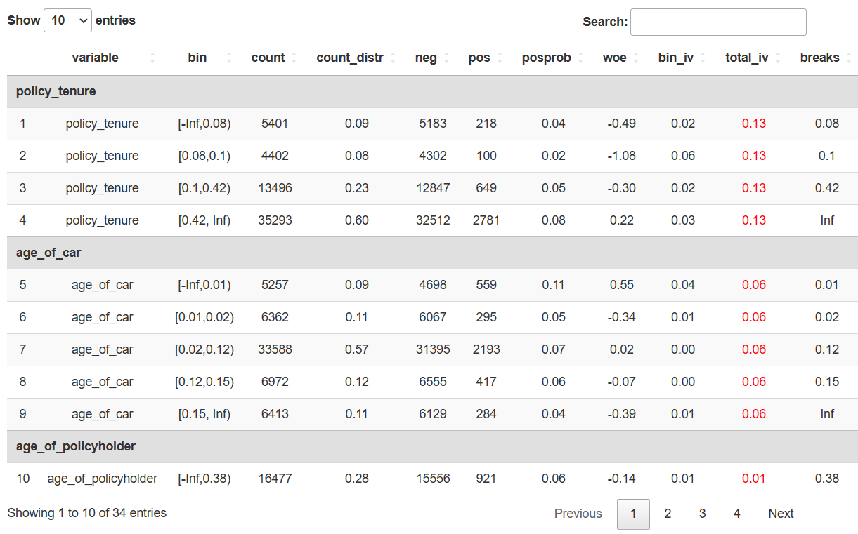
# unique(newbin[total_iv >= 0.01, ]$variable)
feature <-
  c(
    "is_claim",
    "policy_tenure",
    "age_of_car",
    "age_of_policyholder",
    "area_cluster",
    "population_density",
    "f1", "f2", "f3", "f4", "f5")

# 分箱后有些特征的类别仍然较多的话,可以将类别的取值范围接近且 IV 值较小的合并
# 手动调整分箱
break_adj = list(
  age_of_car = c(0.01, 0.02, 0.15),
  population_density = c(15000, 20000, 30000, 40000))

bins_adj = woebin(df[,..feature],
                  y = "is_claim",
                  breaks_list = break_adj,
                  print_info = FALSE)

# 比对一下调整前后的差异
woebin_plot(bins$age_of_car)
woebin_plot(bins_adj$age_of_car)

# WOE转换,得到分箱后的特征
bins_df = data.table::rbindlist(bins_adj)
# 这里的bins_df的格式是数据框,也可以用前面筛选了 IV>0.01 的 newbin
df.woe = woebin_ply(df[,..feature], bins = bins_df, to = 'woe')
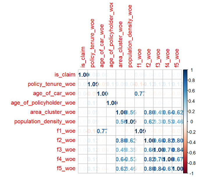
3.2.相关系数 🔗
查看特征之间的相关系数,是为了找出强相关(大于0.85)的特征。笔者的理解是,在高等代数里面,如果一个矩阵里面有完全相等的两列的话,矩阵的行列式等于0,行列式非满秩的矩阵是奇异矩阵,要解方程求解的时候可能会有无穷解或者无解。如果一个矩阵里面存在强相关的特征,也会导致类似情况的发生。为了避免无穷解或无解,强相关的特征要进行删减或转换。
- 在特征数量较少的情况下,可以直接用 corrplot 包的 corrplot 函数来绘制相关系数的图。
library(corrplot)

matrix <- cor(df.woe)
corrplot(matrix, method = "number")
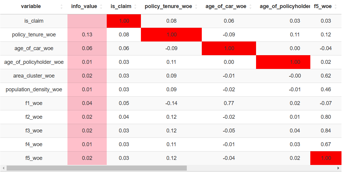
- 但是在特征数量极多的情况下,也可以灵活运用 DT 表格来查看数据。
data.matrix <- as.data.table(matrix)
data.matrix$variable <- colnames(data.matrix)

iv <- iv(df.woe, y = 'is_claim')
data.matrix <- iv[data.matrix, on = 'variable']

datatable(
  data.matrix,
  rownames = FALSE,
  extensions = 'FixedColumns',
  options = list(
    pageLength = 16,
    dom = 't',
    scrollX = TRUE,
    fixedColumns = list(leftColumns = 2, rightColumns = 1),
    columnDefs = list(list(
      targets = '_all',
      className = 'dt-center')))) |>
  formatRound(columns = c(2:13), digits = 2) |>
  formatStyle(columns = c(2),backgroundColor = 'pink')|>
  formatStyle(columns = c(3:13), backgroundColor = styleInterval(c(-0.85, 0.85), c('green', 'white', 'red')))
3.3.逐步回归 🔗
用 bigstep 包的 stepwise 函数做逐步回归来筛选特征。这个包有个限制,一次运行的数据量不能超过100万。
library(bigstep)
library(dplyr)
y <- df.woe%>% pull(is_claim)
x <- df.woe[, -c('is_claim')]
datal <- prepare_data(y, x, type = "logistic")
step_lr <-
  datal %>% reduce_matrix() %>% fast_forward() %>% stepwise()
summary(step_lr)
##
## Call:
## glm(formula = y ~ ., family = binomial(), data = as.data.frame(Xm[,
##     -1]))
##
## Deviance Residuals:
##     Min       1Q   Median       3Q      Max
## -0.6408  -0.4112  -0.3515  -0.2835   3.0102
##
## Coefficients:
##                         Estimate Std. Error  z value Pr(>|z|)
## (Intercept)             -2.68618    0.01743 -154.115  < 2e-16 ***
## policy_tenure_woe        1.07944    0.05643   19.130  < 2e-16 ***
## age_of_car_woe           1.25917    0.07028   17.917  < 2e-16 ***
## f2_woe                   0.81153    0.11520    7.044 1.86e-12 ***
## age_of_policyholder_woe  0.64019    0.16008    3.999 6.36e-05 ***
## ---
## Signif. codes:  0 '***' 0.001 '**' 0.01 '*' 0.05 '.' 0.1 ' ' 1
##
## (Dispersion parameter for binomial family taken to be 1)
##
##     Null deviance: 27860  on 58591  degrees of freedom
## Residual deviance: 27085  on 58587  degrees of freedom
## AIC: 27095
##
## Number of Fisher Scoring iterations: 6
3.4.K折交叉验证 🔗
用 glmnet 包的 cv.glmnet 函数做交叉验证来筛选特征。这个函数默认设置nfolds = 10,即10折交叉验证。
library(Matrix)
library(glmnet)

#生成矩阵和标签
x <-df.woe[,-"is_claim"]
x <- data.matrix(x)
y <- df.woe$is_claim

# 设定随机种子
set.seed(2023)
fit.cv <- cv.glmnet(x, y, family = "binomial", type.measure = "auc")

#查看系数
#plot(fit.cv)
fit.cv$lambda.1se

#去掉系数没有具体数值的特征
coef(fit.cv, s = "lambda.1se")
下面结果中系数有数值的特征,就是筛选出来可以保留的。
## 11 x 1 sparse Matrix of class "dgCMatrix"
##                                  s1
## (Intercept)             -2.66135153
## policy_tenure_woe        0.71153340
## age_of_car_woe           0.65452866
## age_of_policyholder_woe  .
## area_cluster_woe         .
## population_density_woe   .
## f1_woe                   0.19768138
## f2_woe                   0.19161653
## f3_woe                   0.03489065
## f4_woe                   .
## f5_woe                   .
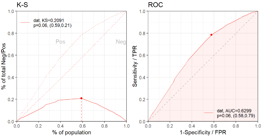
3.5.逻辑回归 🔗
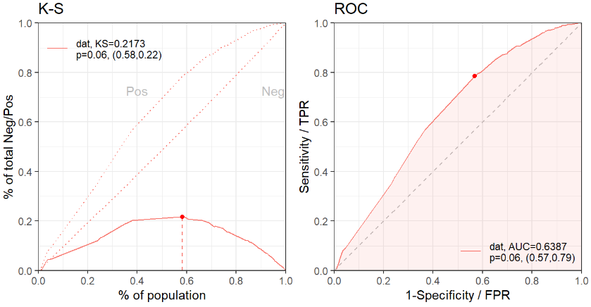
查看用逻辑回归训练的模型基础效果,看看筛选出来的特征是否充分。AUC 值只有0.62,这说明特征是相当不够的。
#正式训练,拆分训练集和验证集
set.seed(2023)
ind <- sample(2, nrow(df.woe), replace = TRUE, prob = c(0.7, 0.3))
train <- df.woe[ind == 1,]
valid <- df.woe[ind == 2,]

#根据逐步回归结果去掉
#根据十折交叉验证结果去掉
#去掉系数显著性检验不通过
#去掉IV值超过0.5的特征
#去掉IV值小于0.02的特征

# 训练
model1 <- glmnet::glm(
  #is_claim ~ policy_tenure_woe + age_of_car_woe + f2_woe + age_of_policyholder_woe
  is_claim ~ policy_tenure_woe + age_of_car_woe + f1_woe + f2_woe + f3_woe
  , family = binomial(link = 'logit'),
  data = train)
summary(model1)

#预测
pred.train <- predict(model1, type = "response", newdata = train)
pred.valid <- predict(model1, type = "response", newdata = valid)

# 训练集
perf.train = scorecard::perf_eva(
  pred = pred.train,
  label = train$is_claim,
  show_plot = c('ks', 'roc'))

# 验证集
perf.test = scorecard::perf_eva(
  pred = pred.valid,
  label = valid$is_claim,
  show_plot = c('ks', 'roc'))
4.训练模型 🔗
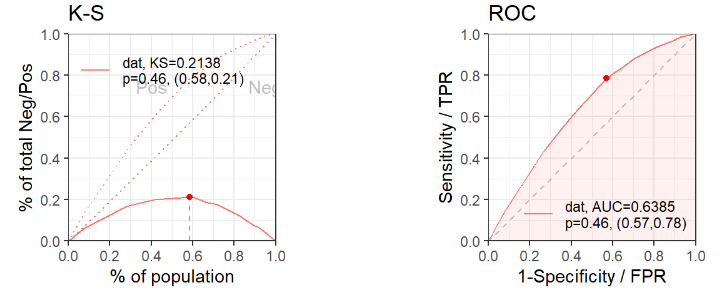
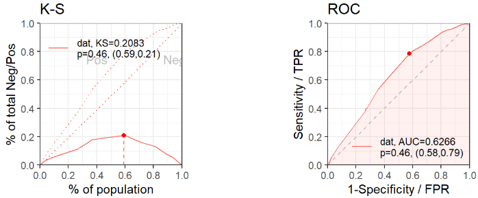
训练模型时会遇到模型过拟合和欠拟合的问题,一般是先减少欠拟合,再减少过拟合。比如,先调整参数使 ROC 曲线下的 AUC 值不断增大,再调整参数使训练集、验证集 KS 值相差不超过0.01。
4.1.调参 🔗
library(xgboost)

##拆分数据集
set.seed(2022)
ind <- sample(2, nrow(df.woe), replace = TRUE, prob = c(0.7, 0.3))
factor <- c('is_claim',
            'policy_tenure_woe',
            'age_of_car_woe',
            'f1_woe',
            'f2_woe',
            'f3_woe')
train <-
  df.woe[ind == 1, ..factor]
valid <-
  df.woe[ind == 2, ..factor]

#拆出训练集和验证集
trainlabel <- train[, 'is_claim']
validlabel <- valid[, 'is_claim']

traindata <- train[,-'is_claim']
validdata <- valid[,-'is_claim']

#若要使用xgb.train,需要先将原来的数据转化为矩阵格式
traindata <- as.matrix(traindata)
trainlabel <- as.matrix(trainlabel)
dtrain <- xgb.DMatrix(data = traindata, label = trainlabel)
validdata <- as.matrix(validdata)
validlabel <- as.matrix(validlabel)
dvalid <- xgb.DMatrix(data = validdata, label = validlabel)

#寻参得到的参数
set.seed(2152)
param1 = list(
  booster = "gbtree",
  objective = "binary:logistic",
  eval_metric = "auc",
  eta = 0.02,
  max_depth = 6,
  min_child_weight = 20,
  gamma = 0.125,
  subsample = 0.89,
  colsample_bytree = 0.51,
  n_estimators = 1000,
  alpha = 0.1,
  lambda = 1,
  verbose = 1)

watchlist <- list(train = dtrain, test = dvalid)
bst1 <-
  xgb.train(
    data = dtrain,
    params = param1,
    nrounds = 1200,
    # nthread = 16, # 默认1,值越大,执行越快
    verbose = 1,
    watchlist = watchlist,
    early_stopping_rounds = 20
  )

#预测结果
pred_train = predict(bst1, newdata = as.matrix(traindata),
                     ntree_limit = 1000)
pred_valid = predict(bst1, newdata = as.matrix(validdata),
                    ntree_limit = 1000)

#训练集
perf.test = scorecard::perf_eva(
  pred = pred_train,
  label = trainlabel,
  show_plot = c('ks', 'roc', 'gain','lift'))

#验证集
perf.test = scorecard::perf_eva(
  pred = pred_valid,
  label = validlabel,
  show_plot = c('ks', 'roc', 'gain','lift'))
4.2.网格寻参 🔗
下面这段寻参代码不记得是在哪里看到,然后笔者只是略微改了一点就拿来用了。寻参过程总是很慢,笔者也许应该去了解一下 foreach、parallel 那些实施并行计算的包,然后来改进这部分的执行效率。
# 寻参时,可不必拆分数据集
train <- df.woe
trainlabel <- train[, 'is_claim']
traindata <- train[, -is_claim]
traindata <- as.matrix(traindata)
trainlabel <- as.matrix(trainlabel)
dtrain <- xgb.DMatrix(data = traindata, label = trainlabel)

best_param = list()
best_seednumber = 1234
# best_logloss = Inf
# best_logloss_index = 0
best_auc = Inf
best_auc_index = 0

for (iter in 1:100) {
  param <- list(
    objective = "binary:logistic",
    # eval_metric = c("logloss"),
    eval_metric = "auc",
    max_depth = sample(5:8, 1),
    eta = runif(1, .01, .3),
    gamma = runif(1, 0.0, 0.2),
    subsample = runif(1, .6, .9),
    colsample_bytree = runif(1, .5, .8),
    min_child_weight = sample(1:40, 1)
  )
  cv.nround = 200 #运行轮次
  cv.nfold = 5
  seed.number = sample.int(10000, 1)[[1]]
  set.seed(seed.number)
  mdcv <- xgb.cv(
    data = dtrain,
    params = param,
    nthread = 16, # 默认1,值越大,执行越快
    nfold = cv.nfold,
    nrounds = cv.nround,
    verbose = T,
    early_stop_round = 8,
    maximize = FALSE
  )

  # min_logloss = min(mdcv[, test_logloss_mean])
  # min_logloss_index = which.min(mdcv[, test_logloss_mean])
  #
  # if (min_logloss < best_logloss) {
  #   best_logloss = min_logloss
  #   best_logloss_index = min_logloss_index
  #   best_seednumber = seed.number
  #   best_param = param
  # }

  min_auc = min(mdcv$evaluation_log[, test_auc_mean])
  min_auc_index = which.min(mdcv$evaluation_log[, test_auc_mean])

  if (min_auc < best_auc) {
    best_auc = min_auc
    best_auc_index = min_auc_index
    best_seednumber = seed.number
    best_param = param
  }
}

best_param
best_seednumber

# nround=best_auc_index
# set.seed(best_seednumber)
# md <-
#   xgb.train(
#     data = dtrain,
#     params = best_param,
#     nrounds = nround,
#     nthread = 16)
4.3.特征重要性 🔗
可以用 xgb.importance 函数查看特征重要性。讲真,笔者也看不懂下面这些数值,只知道 Gain 值自动从高到低排序,代表模型中这些特征重要性逐渐下降。
importance <- xgb.importance(feature_names = colnames(dtrain), model = bst1)
head(importance)
##              Feature       Gain      Cover  Frequency
## 1:    age_of_car_woe 0.36945417 0.44952249 0.45714286
## 2: policy_tenure_woe 0.31074011 0.18814007 0.21428571
## 3:            f1_woe 0.13229080 0.09504380 0.08571429
## 4:            f3_woe 0.12491070 0.18622903 0.17142857
## 5:            f2_woe 0.06260423 0.08106461 0.07142857
刚翻了下xgboost 包最新的文档,可以查看 SHAP 值,还能画图。试了试,报错,不明所以中……笔者对 SHAP 很陌生,连同上网翻的资料一、资料二一并先记在这里,回头再琢磨琢磨单独写一篇。
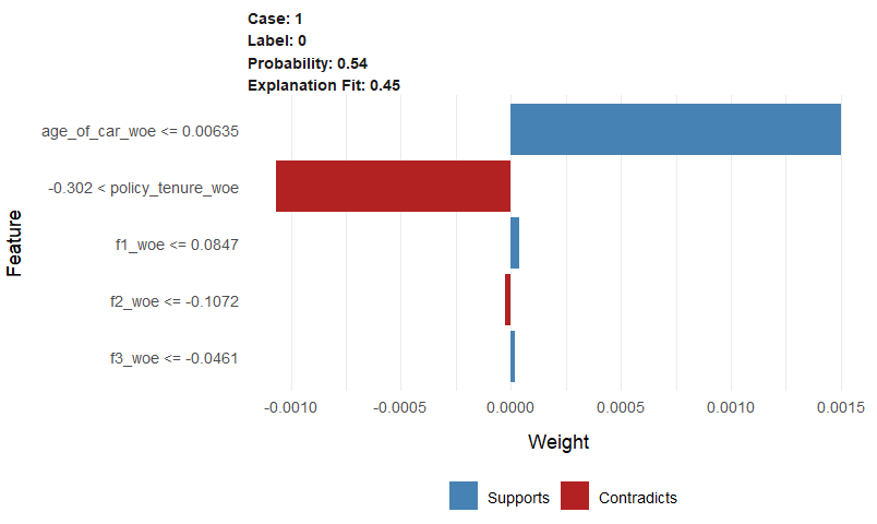
4.4.lime 🔗
用 lime 包可以查看单个样本具体受到哪些特征影响,是正相关还是负相关,影响程度多大等等。
- 蓝色表示正相关,红色表示负相关。
- case 表示样本的序号,Label 是指是否在6月内索赔的结果(1表示是,0表示否)。
- 条形的长度表示特征重要性的大小(即权重,下图中限制仅展示重要性最高的前5个特征)。
需要注意的是,由于 lime 包不一定支持 R 中所有的模型,所以要事先用 model_type 函数检查一下,看需要解释的模型是否被支持。否则,强行解释会报下面这个错。
Error: The class of model must have a model_type method. See ?model_type to get an overview of models supported out of the box.
library(lime)

# 检查前面 xgboost 模型 bst1 是否可以支持
model_type(bst1)

# lime 不支持 xgboost 包的特殊数据格式,得转换成普通数据框
traindata <- as.data.frame(traindata)
explainer <- lime(traindata, bst1)

#查看单个样本
validdata<-as.data.frame(validdata)
explanation <-
  lime::explain(validdata[1,],
                explainer,
                n_labels = 1,
                n_features = 5)

plot_features(explanation)
5.验证 🔗
在建好模型以后,在正式预测之前,需要做一番验证:
-
数据分布是否保持一致。
-
特征是否稳定。假如一个特征在训练集IV值较低,在验证集IV值较高,会导致验证集效果比训练集更好。但是一个特征IV值变化很大是很有风险的,因为不敢确定该特征在未来的测试集上是否依然表现良好。
PSI特征稳定性 🔗
library(scorecard)

pred_list2 = list(pred_train, pred_valid)
names(pred_list2) <- c("train", "valid")
label_list2 = list(train$label, valid)
names(label_list2) <- c("train", "valid")
psi2 = perf_psi(score = pred_list2, label = label_list2)
psi2$psi  # psi data frame

# 分数分布
library(Cairo)
Cairo(
  file = "Cairo_PNG_psi_dpi.png",
  type = "png",
  width = 1200,
  height = 800
)

psi2$pic

dev.off()
IV特征重要性 🔗
iv_train <- iv(train, y = "label")
iv_valid <- iv(valid, y = "label")

colnames(iv_train)[2]<-"iv_train"
colnames(iv_valid)[2]<-"iv_valid"

iv.data <- iv_train[iv_valid, on = "variable"]

iv.data$iv_train_l <-
  ifelse(iv.data$iv_train < 0.02, '无预测力',
         ifelse(iv.data$iv_train < 0.1,'弱',
           ifelse(iv.data$iv_train < 0.3, '中等', '强')))

iv.data$iv_valid_l <-
  ifelse(iv.data$iv_valid < 0.02, '无预测力',
         ifelse(iv.data$iv_valid < 0.1, '弱',
           ifelse(iv.data$iv_valid < 0.3, '中等', '强')))

iv.data
6.预测 🔗
上节建模时设定的目标函数是“binary:logistic”,评价指标是“auc”,预测时输出的结果是概率,即0至1之间的数值。通常在预测概率的基础上再设定阈值,判定好与坏的结果标签。实际业务中设定阈值通常与验证结果所花费的成本相关。若想预测结果直接是0或1,须将目标函数改为“binary:hinge”,评价指标也一并修改。
# 用分箱的结果对测试数据集做 WOE 转换
dtest <- data[type == 'test', ..feature]
dtest.woe = scorecard::woebin_ply(dtest, bins = bins_df, to = 'woe')

# 用训练好的 xgboost 模型 bst1 进行预测
testdata <- as.matrix(dtest.woe[, c('policy_tenure_woe',
                                    'age_of_car_woe',
                                    'f1_woe',
                                    'f2_woe',
                                    'f3_woe')])
pred_test = predict(bst1, newdata = testdata, ntree_limit = 1000)
-
这份数据最奇葩的一点就是,它真的一点都不奇葩。笔者几次三番想换份数据,又无法干脆利落地做到轻易放弃,唉。 ↩︎